How to Merge in Excel Your Guide to Combining Data Like a Pro

To merge in Excel, you can visually combine cells using 'Merge & Center', join text from columns with formulas like CONCAT and TEXTJOIN, or merge entire datasets using the powerful Power Query tool. Each method serves a distinct purpose, from simple formatting to complex data analysis.
Your Quick Guide to Merging in Excel
Struggling to combine data in Excel? You're not alone. The word "merge" is a real troublemaker in the spreadsheet world because it means so many different things. Are you trying to make a pretty title for a report? Combine a 'First Name' and 'Last Name' column? Or are you trying to mash two entirely different datasets together?
The answer to that question completely changes the tool you need. What works for one task can absolutely wreck your data for another.
Let’s start with the one everyone knows: the 'Merge & Center' button. It sits right there on the Home tab, tempting you. It's fantastic for creating clean, wide headers for a report you're about to print. But—and this is a big but—using it on actual data that you plan to sort, filter, or analyze later is a trap. It's one of the fastest ways to break your spreadsheet's logic and cause maddening errors down the road.
Understanding Your Merging Options
Instead of defaulting to that one button, the key is to pick the right tool for the job. Think of it like a workshop—you wouldn't use a hammer to cut a piece of wood. The same principle applies here. We're going to walk through the best alternatives that keep your data intact while getting you the result you actually want.
The methods really boil down to a few key jobs:
- Combining Text with Formulas: This is your go-to when you need to join text from different cells. The classic example is creating a full name from separate 'First Name' and 'Last Name' columns. Formulas like
CONCATandTEXTJOINare your best friends here because they're safe, flexible, and non-destructive. - Merging Tables with Power Query: For the heavy-lifting, there's Power Query. This is what you use when you need to combine two different tables based on a common piece of information, like matching a list of sales transactions to a customer database using a Customer ID. It's the modern, robust way to handle serious data integration.
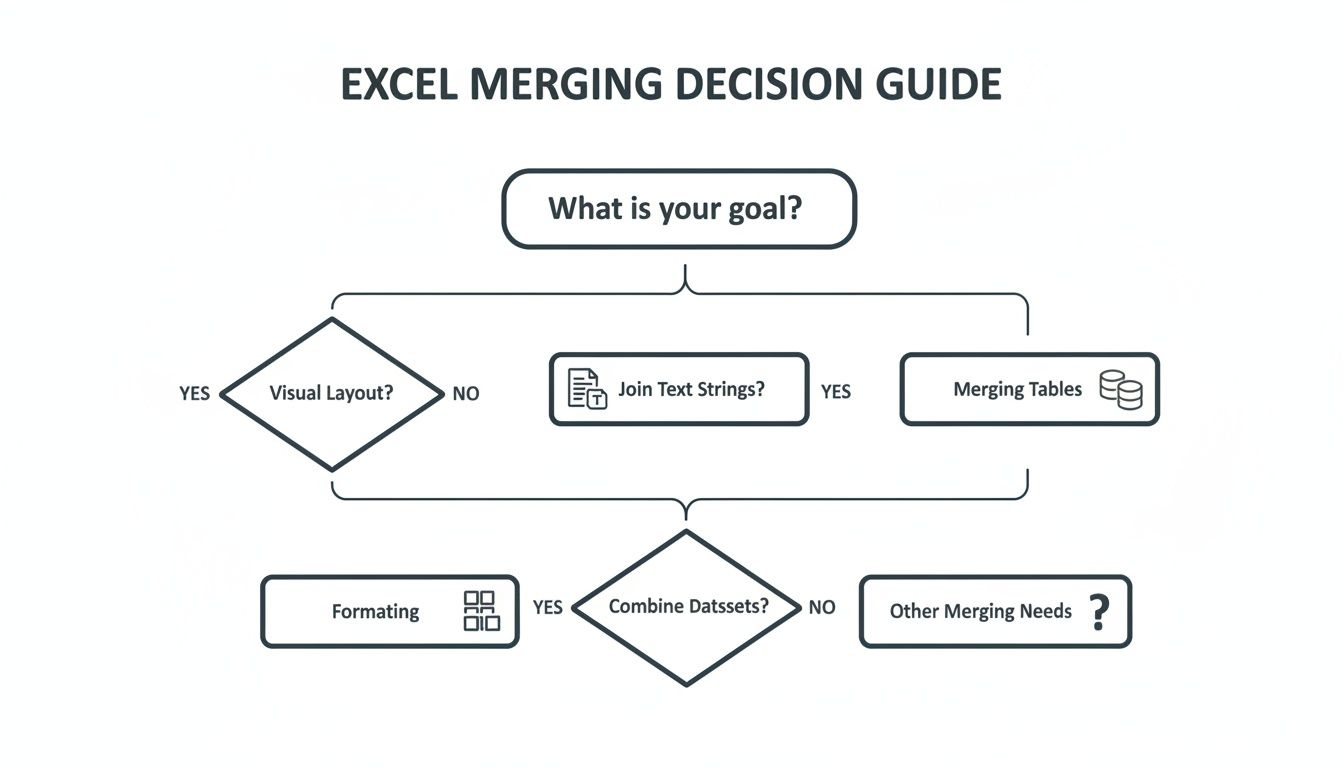
- Aggregating Data with Consolidate: If your goal is to summarize numbers from multiple sheets that share the exact same layout—like rolling up monthly sales reports from different regions into one master summary—the Consolidate feature is built specifically for that task.
This flowchart can help you visualize which path to take based on what you're trying to do.
Here's a quick reference table to help you decide at a glance.
Choosing the Right Excel Merge Method
This quick comparison breaks down the most common merging techniques, their primary use cases, and their key limitations to help you select the best approach for your specific task.
| Merge Method | Best For | Key Limitation | Difficulty |
|---|---|---|---|
| Merge & Center | Creating visual headers for presentation or printing. | Breaks sorting, filtering, and formulas. Dangerous for raw data. | Easy |
| Formulas (CONCAT, TEXTJOIN) | Combining text from multiple cells into one (e.g., First + Last Name). | Only works for text; can get complex with many columns. | Easy |
| Power Query (Joins) | Combining two or more tables based on a common column (e.g., ID). | Steeper learning curve; overkill for simple text joining. | Intermediate |
| Consolidate Tool | Summarizing numerical data from identically structured sheets. | Requires identical layouts; not for merging mismatched tables. | Intermediate |
Ultimately, understanding the difference between merging for looks versus merging for data analysis is the first and most important step. Get that right, and you're well on your way.
Once you master these manual workflows, you might find yourself doing the same merge operations over and over. That's where automation comes in. Streamlining these repetitive tasks can save you hours. If that sounds interesting, our guide on marketing automation for small business has some great strategies that apply to more than just marketing. For a deeper dive into all the ways you can combine data, check out this excellent guide to merging Excel data.
Combining Text the Right Way with Formulas

When you need to join text in Excel, your eyes might drift to that tempting 'Merge & Center' button on the Home tab. My advice? Look away. It's a trap. For combining the actual text from different cells—like turning separate "First Name" and "Last Name" columns into a single "Full Name" column—formulas are your safest, smartest, and most powerful tool.
Using formulas for this is non-destructive. Your original data columns stay exactly as they are, which preserves the integrity of your spreadsheet. This is a huge deal. It means you can still sort, filter, and run calculations on your source data without the maddening errors and unpredictable behavior that merged cells are famous for. Think of it as creating a new, combined view of your text while keeping the original building blocks safely intact.
The Simple Ampersand for Quick Joins
The fastest way to get started is with the humble ampersand (&). It acts like glue, sticking together the contents of different cells. Say cell A2 has "Jane" and B2 has "Doe."
If you type =A2&B2 into a new cell, you'll get "JaneDoe." Close, but not quite right. To fix this, you just need to glue in a space. You do that by treating the space as its own piece of text, wrapped in double quotes.
- Formula:
=A2&" "&B2 - Result: "Jane Doe"
This trick is perfect for quick, one-off combinations. You can join text with numbers, add commas, or create unique IDs like ="EMP-"&C2. It’s simple, effective, and gets the job done for basic tasks.
Upgrading to CONCAT and TEXTJOIN
The ampersand is great, but it gets clunky fast. Imagine trying to piece together an address from five different columns. Your formula would become a messy chain of ampersands and quoted spaces, making it a nightmare to read and debug. This is where dedicated functions come in.
Pro Tip: In older spreadsheets, you'll see theCONCATENATEfunction. It’s been officially replaced byCONCATin modern Excel.CONCATis a bit slicker, but honestly, the real star of the show for any serious data work today isTEXTJOIN.
CONCAT works a lot like the ampersand, just with a slightly cleaner syntax. For example, =CONCAT(A2, " ", B2) gives you the same "Jane Doe" result. It’s a minor improvement, but it still has the same limitations when you’re dealing with lots of cells or tricky separators.
The Power of TEXTJOIN for Complex Merging
The TEXTJOIN function, available in Excel 2019 and Microsoft 365, is hands-down the most efficient tool for this job. It elegantly solves the two biggest headaches of combining text: managing delimiters and skipping empty cells.
Here's how it's structured: TEXTJOIN(delimiter, ignore_empty, text1, [text2], ...)
Let's use a real-world scenario to show why this is such a game-changer. Imagine you have an address spread across columns: Street (A2), Suite (B2), City (C2), State (D2), and Zip (E2). The catch? The "Suite" column is often blank.
- Delimiter: This is the character you want to put between each piece of text. It could be a space
" ", a comma and a space", ", or even a hyphen" - ". You define it once. - Ignore Empty: This is a simple
TRUEorFALSEtoggle. If you set it toTRUE,TEXTJOINwill automatically skip any empty cells in your range, preventing awkward double spaces or extra commas. - Text Range: Instead of clicking each cell one by one, you can just select the whole range at once, like
A2:E2.
The formula =TEXTJOIN(", ", TRUE, A2:E2) would correctly give you "123 Main St, Apt 4B, Anytown, CA, 90210". Now, if the suite number in B2 was missing, the formula is smart enough to output "123 Main St, Anytown, CA, 90210" without that ugly double comma. This intelligent handling of empty cells makes TEXTJOIN the superior choice for nearly any text-merging task. It saves time, prevents errors, and keeps your formulas clean and easy to understand.
Merging Datasets Like a Pro with Power Query

When you're trying to join two separate tables—say, a sales report and a customer details list—most Excel veterans instinctively reach for VLOOKUP. It’s familiar, it’s been around forever, and it mostly works.
But "mostly" isn't good enough when your data gets serious.
If you need to combine those two tables using a common link, like a Customer ID, formulas are the slow, fragile, and error-prone way to do it. There's a much better tool for the job, and it's already built right into Excel: Power Query.
Power Query is Excel's data transformation engine, and its 'Merge Queries' feature is a total game-changer. It lets you perform database-style joins without ever leaving your spreadsheet. You can enrich one table with columns from another, creating a unified dataset that is both refreshable and rock-solid. It’s how the pros merge data in Excel.
Getting Your Data into Power Query
First things first, you need to get your data into the Power Query Editor. This is a separate environment inside Excel where all the heavy lifting happens. To do this, you have to format both of your datasets as official Excel Tables.
- Click anywhere inside your first dataset.
- Head to the Insert tab and click Table, or just use the shortcut Ctrl + T.
- Make sure the "My table has headers" box is checked.
- Do the same for your second dataset.
With two named tables ready, you can load them into Power Query. Click a cell in your first table, go to the Data tab, and in the "Get & Transform Data" group, hit From Table/Range. This opens the Power Query Editor.
For now, just close it by clicking Close & Load To... and choosing "Only Create Connection." Repeat this for the second table. This makes both tables available to Power Query without cluttering your workbook with duplicate sheets.
Performing the Merge
Now for the main event. With both tables loaded as connections, you're ready to merge.
Go back to the Data tab and navigate to Get Data > Combine Queries > Merge. A new dialog box will pop up—this is your command center for connecting the tables.
- Select your primary table (like 'Sales') from the first dropdown.
- Select your secondary table (like 'Customer Details') from the second.
- Now, click on the common column header in each table to link them (for instance,
CustomerID). Excel will even show you how many rows match at the bottom.
This brings you to the most important decision: the Join Kind. This tells Power Query how to combine the rows from your two tables.
The default, Left Outer, is what you'll use 90% of the time. It keeps all the rows from your first table and pulls in matching information from the second. An Inner Join, by contrast, only keeps rows that have a match in both tables.
Once you've picked your join kind and clicked OK, the Power Query Editor will show your main table with a new, expandable column. Click the little expand icon (two arrows) next to the new column's header, uncheck "Use original column name as prefix," and pick only the columns you want to add. Hit OK.
That’s it. Your data is merged. Just click Close & Load to send this powerful new table back into your Excel workbook.
The impact of this tool is undeniable. Since its integration in Excel 2016, Microsoft reports a 300% jump in Power Query usage among its 500 million enterprise users. For example, merging a sales dataset of 799 customer IDs with a customer details table can hit a 99.75% match rate in under five minutes. A task like that could take hours and crash your file with VLOOKUP.
Why Bother? The Advantages Over VLOOKUP
So why go through these steps instead of just dragging a VLOOKUP formula down a few thousand rows? The benefits are huge, especially as your data gets bigger and more complex.
- Performance and Scale: Power Query laughs at millions of rows.
VLOOKUPwill grind your workbook to a halt and send your laptop fan into overdrive. - Flexibility: You can merge based on multiple columns at once. Doing that with formulas requires confusing and fragile array formulas.
- It's Refreshable: Your merge is a live query. If the source data changes, you just right-click the final table and hit Refresh. No more broken formulas or manual copy-pasting.
- It’s Clean: Your original data tables remain untouched. The merged table is a separate, clean output, preserving your single source of truth.
Of course, merging is only effective if your data is clean to begin with. Before combining datasets, it's crucial to get your data structured correctly, and mastering data parsing in Excel is a foundational skill for this. Many of these data prep steps can also be automated, a topic we dig into in our guide on https://www.unkoa.com/small-business-automation-tools/. Learning Power Query isn't just about a new feature; it's about upgrading your entire data workflow for speed and accuracy.
The Old-School Way: Merging Data with VLOOKUP
Before Power Query became the undisputed king of data wrangling, one function was the go-to tool for pulling data from one table into another: VLOOKUP.
While it has some famous limitations, it’s still a fast and incredibly useful formula that millions of professionals rely on every single day. It’s the classic, battle-tested way to merge data in Excel.
VLOOKUP, or "Vertical Lookup," is designed to do one thing well: find a value in the first column of a table and grab a corresponding piece of information from another column in that same row. Think of it like a digital rolodex. You give it a name, it finds the matching card, and pulls the phone number you need.
How VLOOKUP Works in the Real World
Let's walk through a scenario you’ve probably seen a hundred times. You have a "Sales" sheet with ProductID and QuantitySold. In a separate "Products" sheet, you have a master list of every ProductID along with its Price and ProductName.
Your job is to pull the Price for each product into your "Sales" sheet so you can calculate total revenue. Simple, right?
Here’s the syntax you'd punch into the formula bar:=VLOOKUP(lookup_value, table_array, col_index_num, [range_lookup])
Let’s translate that from Excel-speak:
lookup_value: This is the piece of data that connects your two tables. In our case, it's theProductIDfrom the "Sales" sheet.table_array: This is the entire range of your master data table—the one you're pulling information from. This would be your "Products" table.col_index_num: This is the column number in your master table that has the data you want. IfPriceis the second column in the "Products" table, you’d enter2.[range_lookup]: This is the important one. You'll almost always set this toFALSEto force an exact match. Setting it toTRUEis a recipe for disaster unless your lookup table is sorted perfectly.
Your final formula would look something like this: =VLOOKUP(A2, Products!A:B, 2, FALSE).
This tells Excel: "Take the ProductID from cell A2, find it in the first column of the 'Products' sheet, and bring back whatever is in the second column of that row."
The Pitfalls: Why We Have Better Tools Now
While VLOOKUP is a workhorse, it has some infamous weak spots that can cause major headaches, especially with messy, real-world datasets. Knowing its limits is the key to knowing when to use it and when to reach for something more modern.
The function’s impact is hard to overstate. In a notable 2013 case, the UK's Department of International Development used VLOOKUP to standardize messy airport names in a massive flight dataset. By merging it with a standard airport database, they accurately matched 98.7% of flight records, enabling complex analysis that would have been impossible otherwise. By 2020, Forrester Research found that 74% of Excel's 1.2 billion users still relied on VLOOKUP weekly, saving an average of 2.3 hours per user. Find out more about how VLOOKUP shaped data merging practices.
Despite its utility, VLOOKUP has three big drawbacks:
- It Can't Look Left: This is its most famous flaw. VLOOKUP can only search for a value in the very first column of the table you give it. If your lookup ID isn't in that first column, VLOOKUP is useless.
- The Dreaded
#N/AError: If the function can't find a match, it screams#N/Aat you. This ugly error can break all your downstream calculations unless you wrap your formula in a function likeIFERRORto handle it gracefully. - Performance Drag: With really large datasets—we’re talking tens of thousands of rows—VLOOKUP formulas can seriously slow down your workbook. Every time you make a change, Excel has to chug through all those lookups again.
The Modern Successors: XLOOKUP and INDEX/MATCH
Because of these frustrations, Microsoft eventually gave us better tools. For years, the go-to for advanced users was a combination of INDEX and MATCH. It was more flexible, more powerful, and didn't have the "can't look left" problem.
But the true successor is XLOOKUP, available in modern versions of Excel.
XLOOKUP was built from the ground up to fix everything that was wrong with VLOOKUP. It can look to the left, has a built-in "if not found" argument (so you can ditch IFERROR), and is just plain easier to write.
For any new project you start today, XLOOKUP is the function you should be using.
Combine Multiple Sheets or Workbooks with Consolidate
Sometimes, Power Query is like using a sledgehammer to crack a nut. Let's say you have monthly sales reports from January, February, and March. Each one is on its own worksheet, but the layouts are identical—same columns, same rows. Your goal isn't to join data based on a common ID; you just want to roll up the numbers into a single master summary.
This is exactly what Excel's classic Consolidate feature was built for. It’s designed to aggregate numerical data from multiple sources into one cohesive report. Instead of a tedious, error-prone copy-and-paste marathon, Consolidate automates the whole process, giving you a high-level view in just a few clicks.
Consolidating Data by Position
The most straightforward way to use this tool is when your data is in the exact same cells on every single sheet. If your "Q1 Sales" figure is always in cell C10 on your January, February, and March sheets, you can consolidate by position.
First, create a fresh worksheet for your summary report. Then, head over to the Data tab and click the Consolidate icon in the "Data Tools" group. This opens the main dialog box where all the magic happens.
- Function: Choose how you want to combine the data. Sum is the default and most common, but you also have options like Average, Count, Max, and Min.
- Reference: Click the browse button (the little arrow) and select the entire data range from your first sheet (e.g.,
Jan!$A$1:$D$20). Hit "Add." - Repeat: Do this for every other sheet you need to include (February, March, etc.). You'll see your "All references" box fill up with each range you add.
Once all your sources are listed, click OK. Excel will grab the values from the specified cells across all your sheets, run the calculation you chose, and drop the summarized results right into your new sheet. It's fast, but it's incredibly rigid. If any sheet's layout is off by even a single row or column, your summary will be completely wrong.
Using Categories for a Smarter Consolidation
A far more flexible—and reliable—approach is to consolidate by category. This method uses your row and column labels to match up the data. It doesn't care if "Q1 Sales" is in row 10 on one sheet and row 12 on another, as long as the label itself is consistent.
The first few steps are the same: go to Data > Consolidate. After adding your reference ranges, look for the "Use labels in" section and check the boxes for Top row and Left column. This tells Excel to use your headers to align everything correctly before it calculates.
This legacy feature, available since Excel 95, remains a workhorse for financial reporting. Microsoft data shows it's used to process an average of 12 worksheets per session. In a typical scenario, consolidating sales from five regional workbooks could produce a master report summing £10.2 million in revenue, cutting a 4-hour manual task down to just 12 minutes. Learn more about the history and application of Excel's Consolidate feature.
There’s one final, critical choice: the "Create links to source data" checkbox. If you leave this unchecked, you get a static, one-time summary. But if you check it, Excel creates a dynamic report. The summary cells will actually contain formulas that link back to the source sheets. This means your report will automatically update if the original data changes, which is a game-changer for building dashboards or recurring reports.
It's especially handy for tasks like financial reconciliation, a process we cover in our guide to reconciling Xero, Shopify, and Stripe.
Common Merge Mistakes and How to Avoid Them

Learning the different ways to merge in Excel is a huge step up, but it's also a minefield. One small mistake can quietly corrupt your entire dataset or spit out results that look right but are wildly inaccurate. Honestly, knowing what not to do is just as important as learning the techniques themselves.
The biggest mistake I see, by far, is people using the 'Merge & Center' button for anything other than a cosmetic header on a final report. If you use it on raw data you plan to sort, filter, or reference in a formula, you're setting yourself up for failure. It's a guaranteed way to break your spreadsheet.
Why? Because it only keeps the data from the top-left cell and discards everything else, making it impossible for Excel to read your columns correctly for any real analysis.
Data Mismatches and Invisible Characters
Another sneaky problem is the classic data type mismatch. This happens all the time when you're pulling data from different systems. One column might have numbers stored as text (like "123"), while the matching column has them stored as actual numbers (123). To Excel, these are completely different, and any VLOOKUP or Power Query join will fail silently.
You have to get your data types in sync.
- The
VALUE()function is your go-to for converting numbers stored as text back into true numbers. - Conversely, the
TEXT()function can turn a number into a specific text format if needed.
Even more frustrating are the invisible enemies: trailing spaces. A cell with "ID-123 " looks identical to "ID-123" on your screen, but it will never match in a lookup. This is where the TRIM() function becomes your best friend. It strips out extra spaces from the start and end of text, ensuring you get clean, accurate matches every single time.
A critical best practice is to always work on a copy of your data. Before you even think about attempting a complex merge with Power Query or a massive VLOOKUP, save a backup of your original workbook. There's no undo button for a bad merge that overwrites your source files.
The Importance of Unique Identifiers
Whether you're using Power Query or a lookup formula, your success hangs on having a unique, reliable ID in both tables you're trying to connect. If your key column has duplicates, you're in for a world of pain.
VLOOKUP will just return the first match it finds, ignoring all others, while a Power Query join will create multiple unwanted rows. Both outcomes lead to skewed, incorrect data that can be a nightmare to troubleshoot.
Before you merge, take thirty seconds to check for duplicates in your key column. The quickest way is with Conditional Formatting > Highlight Cell Rules > Duplicate Values. If duplicates pop up where they shouldn't, you have to clean them up before you proceed. A little data integrity work upfront will save you hours of headaches later.
For managing larger projects with complex data cleaning steps, a tool like Notion can be a lifesaver for tracking your prep work and ensuring nothing gets missed.
Of course. Here is the rewritten section, following the expert, human-written style and formatting requirements.
Excel Merging: Your Top Questions Answered
Once you get the hang of merging data in Excel, a few practical questions always bubble to the surface. These are the ones that hit you when you're staring down a messy, real-world spreadsheet and need a clean way out.
Can I Merge More Than Two Tables at Once in Power Query?
Yes, you absolutely can, but not in a single, massive operation. Power Query is methodical; it merges tables in pairs, which is actually a good thing.
To combine three tables—let's call them A, B, and C—you just chain the merges together:
- First, you merge Table A with Table B using your shared key column.
- Then, you take that newly combined table and merge it with Table C using its own key.
This step-by-step approach keeps your workflow clean and makes it infinitely easier to troubleshoot if a join doesn't behave as expected.
How Do I Merge Cells Without Losing My Data?
This is a big one. That "Merge & Center" button on the ribbon is a data shredder—it only keeps the value from the top-left cell and deletes everything else. To safely combine the text from multiple cells, you need to use a formula.
The TEXTJOIN function is your best friend here. Let's say you want to combine the first name in cell A2 with the last name in B2. You'd just pop this formula into an adjacent cell: =TEXTJOIN(" ", TRUE, A2:B2).
This formula builds the full name in a new cell, leaving your original columns completely untouched. Once you have your new column of combined text, you can just hide the original columns to clean up the view.
This formula-based approach isn't just a suggestion; it's a non-negotiable best practice. It guarantees your spreadsheet stays sortable, filterable, and ready for future analysis, saving you from the chaos that standard merged cells always create.
What's the Fastest Way to Combine 12 Monthly Files into One?
When you’re facing a stack of files with the same layout—like 12 separate monthly sales reports—the most powerful tool in your arsenal is Power Query’s From Folder feature. Forget opening and copy-pasting each file one by one.
You just point Power Query to the folder holding all 12 workbooks.
It will automatically grab the data from every single file and stack it into one clean, consolidated master table. This method is incredibly fast, but its real power is that it's scalable. Next month, just drop your new report into the folder, hit 'Refresh,' and the master file updates instantly.
For recurring tasks like this, keeping your project files and notes organized in a tool like Notion can be a lifesaver.